The VEV Calculation – More Detail

This section outlines the process of calculation of the VaR Equivalent Volatility (VEV) which is used in the calculation of MRM for Category 2 PRIIPs.

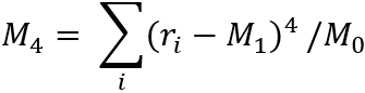
This calculation embraces the concept of the Cornish-Fisher Expansion method which transforms the Value at Risk (VaR) calculation into a volatility risk measure.

Once calculated, this VaR Equivalent Volatility (VEV) number is then assigned to a market risk measure (MRM) category ranging from a scale of 1 to 7. For example, a VEV of 10% would place the security into an MRM Class of 3.

An MRM Class of 1 contains those securities with the lowest risk, while a class of 7 would indicate the highest risk category.

CALCULATED ANNUALISED VEV	MRM CLASS
< 0.5%	1
0.5% - 5.0%	2
5% - 12%	3
12% - 20%	4
20% - 30%	5
30% - 80%	6
> 80%	7

The section below takes you through the required steps from manipulating the history of observed returns to calculate the Value at Risk (VAR) and finally calculating the VaR Equivalent Volatility (VEV).

BACKGROUND INFORMATION

To complete the calculation of the VEV you should ensure you have an understanding of the below key terms before carrying out the calculation.

Cornish-Fisher Expansion – It is a formula for approximating the quantiles of a random variable based only on its first few “moments”.

Moments – Provide statistical information of the shape of the distribution. For example:

The zero moment is the count of the number of observed returns in the period
The first moment is the mean (calculated by summing all the returns and dividing them by the number of returns)
The second moment is the variance
The third moment provides information on skewness of a distribution
The fourth moment provides information relating to the kurtosis of a distribution.

HOW TO CALCULATE THE SECOND, THIRD AND FOURTH MOMENTS

Below is a summary of how to calculate the second, third and fourth moments, using the second moment as an example.

2ND MOMENT:

Take each individual return and subtract the mean (M_1) from it. Then sum this.
The value in step 1 is then taken to the power of the required moment, for example the second moment would be calculated by squaring the result.
Next divide the result by the number of observed returns in the period (M_0).

This is the second moment.

3RD MOMENT:

The third moment calculates the skewness of the observed returns in the period.

4TH MOMENT:

The fourth moment calculates the kurtosis of the observed returns in the period.

VOLATILITY (σ)

A statistical measure of dispersion of returns for a given security or market index. It can be calculated using the standard deviation or the variance and typically the higher the volatility the riskier the security.

SKEWNESS

A measure of symmetry or lack of symmetry that is used to describe the distribution of a dataset. It provides a measure of the variance of a dataset relative to a Normal Distribution (i.e. where all data is symmetric and distributed equally around the mean). A dataset is skewed if the points are not symmetrical, for example, positive skew occurs if the right tail of the distribution is longer than the left. A symmetrical distribution will have 0 skewness.

KURTOSIS

A statistical measure as to whether the data is heavily-tailed or light-tailed relative to a normal distribution. A heavily tailed graph suggests a high presence of outliers (data which doesn’t fit in with the other data) whereas a light tailed graph tends not to have any outliers.

EXCESS KURTOSIS

The kurtosis for a standard normal distribution is three, therefore we calculate the excess kurtosis as the Kurtosis -3. We do this so the that the standard normal distribution has a kurtosis of zero.

This is an important consideration to take when examining historical returns from a stock or portfolio. For example, the larger the kurtosis coefficient is compared to the normal distribution means that the future returns will be either extremely large or small.

WHY USE THE NORMAL DISTRIBUTION?

There is a strong correlation between the size of a sample and the extent to which a sampling distribution approaches a normal form. For example, we could have a large set of N returns which are normally distributed.

In the calculations below, we take the value of -1.96 within both the VaR and VEV formula. This value of -1.96 is the inverse normal for the 97.5th percentile which comes from the table of standardised normal values. As we are looking at the inverse-normal we take 1 – percentile. Therefore, in this case we look at the 2.5th percentile in order to obtain our z value of -1.96. This table is a standard mathematical table and is widely available online). It is also built into the calculation tools, including Microsoft Excel.

STEP 1: HISTORY OF OBSERVED RETURNS

The return over each period is defined as the natural logarithm of the ratio of the price at the market close at the end of the current period to the market close at the end of the preceding period. Natural logarithms are used as the calculation is based on continuous returns, and not discrete or linear returns. It is important to note that this is not the same as calculating the percentage change.

Returns should only be calculated for periods post-launch for dates on which the shareclass issues a price. This means that returns do not need to be calculated and included for bank holidays or other non-pricing dates.

In order to calculate the “history of observed returns” of the PRIIP:

Take the price at the end of the current period and divide this by the price at the end of the previous period.
Take the natural logarithm of this value.
From this information we can also calculate the mean return and the number of days within the period.

For example:

Notes:

If you have a positive return of 0.015 and a negative return of -0.014, the average is going to be 0.005, therefore you will end up with some very small numbers;
The natural logarithm returns are not made absolute, which means that the mean can be a negative value.

ESMA regulations advise that:

“VaR shall be calculated from the moments of the observed distribution of returns of the PRIIP’s or its benchmark or proxy’s price during the past 5 years. The minimum frequency of observations is monthly. Where prices are available on a daily basis, the frequency shall be daily. Where prices are available on a weekly basis, the frequency shall be weekly. Where prices are available on a bi-monthly basis, the frequency shall be bi-monthly.

Where data on daily prices covering a period of 5 years are not available, a shorter period may be used. For daily observations of a PRIIP’s or its benchmark or proxy’s price, there shall be at least 2 years of observed returns. For weekly observations of a PRIIP’s price, there shall be at least 4 years of observed data. For monthly observations of a PRIIP’s price, there shall be observed data covering a period of at least 5 years.”

It should be borne in mind that the above are minimums and that all efforts should be made to ensure that the full 5 years of data is sourced and used in the relevant calculations. In reality, there are very few scenarios whereby proxy or benchmark data is not available, given the multiplicity of benchmarks available in the marketplace. The use of less than 5 years data does render the end calculations less reliable and more prone to fluctuations in particular for stress and favourable performance scenario calculations.

Click here for more information.

STEP 2: VALUE AT RISK RETURN SPACE

ESMA use the phrase “VAR Return Space.” ESMA define this as VAR calculated using the Cornish Fisher expansion method. “VAR Return Space” is an ESMA term, not a not a known mathematical concept. In contrast “VAR calculated using the Cornish Fisher expansion method” is a known concept.

The VaR is calculated using the Cornish Fisher Expansion as follows:

Where:

N = the number of trading periods in the specified period.
σ = √(M_2 )
This is the volatility. As we can see from the below formula for the second moment, M2, the volatility is the square root of the variance.
μ_1= M_3/σ^3
This is the skew. The third moment, M3, is divided by the volatility cubed.
μ_2=M_4/σ^4 -3
This is the excess kurtosis. It uses the fourth moment, M4, and divides it by the volatility to the power of four.
-1.96 is the inverse normal for the 97.5th percentile. This is determined by the normal distribution Z tables.
The other values are constant values taken from the Cornish Fisher Expansion.

The references to M2, M3, M4 are references to the second, third and fourth moments – see above.

As above, the volatility, skew and excess kurtosis can be calculated from the measured moments of the distribution of returns as follows, where r_i is the return measured on the ith period in the history of returns.

STEP 3: VAR EQUIVALENT VOLATILITY (VEV)

To calculate the VaR Equivalent Volatility (VEV) we use the result from the VaR Return Space formula above along with other constants and ‘T’ which is the length of the holding period in years. Using this expansion allows the VaR number to be transformed into a volatility-like measure (VEV).

The VEV is given by:

Where:

T is the length of the holding period in years.
VaRRETURN is the Value at Risk (VaR) over a period of time.

The result from the VEV formula is the annualised volatility. We can then assign an MRM Class based off the output.

Example:

If we take the values as follows:

VARIABLE	VALUE
VaR Return Space	0.05
T	4

Then the calculation would be:

This would then be multiplied by 100 to get it as a percentage, i.e. 66.7%.

Having regards to PRIIPs, as we can see in the table at the start of the document, a VEV of 66.7% would give it a market risk measure (MRM) category of 6.